Global leaf size analysis

Introduction

This post was originally written as a response to Wright et al., 2017, and is supplemental to the eLetter we wrote in response to that acticle.

Overview

In a break from Wright et al., we used the more recent approach to calulating R² for mixed model from Nakagawa & Schielzeth 2013 as implemented in the MuMIn package.

The Nakagawa and Shielzeth method calculates a marginal R² that shows the proportion of variation attributable to fixed effects only (analagous to those reported by Wright et al.), and also a conditional R² that shows the total variation explained by the model (both fixed and random effects)

### Load Packages
require(ggplot2) # Needed for plotting
require(cowplot) # Needed for publication-quality ggplots
require(dplyr) # Needed for data wrangling
require(readxl) # Needed to read in the Excel file
require(lme4) # Needed for mixed modelling
require(MuMIn) # Needed for R^2 calculation
require(knitr) # Needed to print out tables
require(readxl) # Needed to read in excel files


### Import a function to make a nice table with AIC and R^2
source("AIC.R2.table.R")

### Import the Wright et al. dataset

# Specify the Science URL for the Wright et al. dataset
# NOTE: if this doesn't work, use read_excel() to import the dataset directly.
dataURL <- "http://science.sciencemag.org/highwire/filestream/698792/field_highwire_adjunct_files/1/aal4760-Wright-SM_Data_Set_S1.xlsx"

# Download the xlsx dataset and read into R
tmpfile <- tempfile(fileext = ".xlsx")
download.file(dataURL, tmpfile, mode = "wb")
data <- read_excel(path = tmpfile, sheet = "Global leaf size dataset")

# Clean up the dataset
global <- data %>% 
    
    # Select columns: family, species, site, size, latitude, & climate variables
    select(Family, Species = `Genus species`, Site = `Site name`, 
        Leaf.size = `Leaf size (cm2)`, Latitude, MAT, MAP, MIann, 
        Tgs, RADann, Compound_Simple) %>%
    
    # Filter out all rows without a leaf size
    filter(!is.na(Leaf.size))

# Show dataset structure
#str(global)

##### Random Effect Models ##### 

# Model with Site + Species random effects
sitesp <- lmer(log10(Leaf.size) ~ (1|Site) + (1|Species), data = global)

# Model with Family random effect
family <- lmer(log10(Leaf.size) ~ (1|Family), data = global)

# Model with Site + Family + Species random effects
sitefamilysp <- lmer(log10(Leaf.size) ~ (1|Site) + (1|Family) + (1|Species), 
    data = global)

Latitude

The best model for explaining latitudinal gradients in leaf size includes Site, Species, and Family as random effects. Models with family alone outperform models that include Latitude without random effects. In the model used by Wright et al., with species and site as random effects, most of the variance was explained by these random effects, rather than latitude.

##### Latitude Models ##### 

# Full Wright et al. model: Latitude + Site + Species
lat.m1 <- lmer(log10(Leaf.size) ~ poly(Latitude, 2, raw = TRUE) + 
    (1|Site) + (1|Species), data = global)

# Full Wright et al model with Family: Latitude + Site + Family + Species
lat.m2 <- lmer(log10(Leaf.size) ~ poly(Latitude, 2, raw  = TRUE) + 
    (1|Site) + (1|Family) + (1|Species), data = global)

# Model with only Latitude: no random effects
lat.m3 <- lm(log10(Leaf.size) ~ poly(Latitude, 2, raw  = TRUE), data = global)

# Make a table with AIC and Marginal and Conditional R^2
lat.tbl <- AIC.R2.table(lat.m1, lat.m2, lat.m3, sitesp, family, sitefamilysp, 
    mnames = c("Latitude + Species + Site (Wright)", 
        "Latitude + Site + Family + Species", "Latitude", "Site + Species", 
       "Family", "Site + Family + Species"))

# Print out a markdown table
kable(lat.tbl, format = "markdown")

Model	AIC	dAIC	df	R2.marg	R2.cond
Latitude + Site + Family + Species	14986.72	0.00	7	0.171	0.948
Site + Family + Species	15386.82	400.10	5	0.000	0.947
Latitude + Species + Site (Wright)	16538.27	1551.54	6	0.231	0.945
Site + Species	16948.59	1961.87	4	0.000	0.945
Family	29081.79	14095.06	3	0.000	0.481
Latitude	30835.92	15849.20	4	0.282	0.282

MAP

##### MAP Models ##### 

# Full Wright et al. model: MAP + Site + Species
map.m1 <- lmer(log10(Leaf.size) ~ MAP + 
    (1|Site) + (1|Species), data = global)

# Full Wright et al model with Family: MAP + Site + Family + Species
map.m2 <- lmer(log10(Leaf.size) ~ MAP + 
    (1|Site) + (1|Family) + (1|Species), data = global)

# Model with only MAP: no random effects
map.m3 <- lm(log10(Leaf.size) ~ MAP, data = global)

# Make a table with AIC and Marginal and Conditional R^2
MAT.tbl <- AIC.R2.table(map.m1, map.m2, map.m3, sitesp, family, sitefamilysp, 
    mnames = c("MAP + Species + Site (Wright)", 
        "MAP + Site + Family + Species", "MAP", "Site + Species", 
       "Family", "Site + Family + Species"))

# Print out a markdown table
kable(MAT.tbl, format = "markdown")

Model	AIC	dAIC	df	R2.marg	R2.cond
MAP + Site + Family + Species	15305.31	0.00	6	0.051	0.947
Site + Family + Species	15386.82	81.51	5	0.000	0.947
MAP + Species + Site (Wright)	16859.78	1554.46	5	0.076	0.945
Site + Species	16948.59	1643.28	4	0.000	0.945
Family	29081.79	13776.47	3	0.000	0.481
MAP	33228.50	17923.18	3	0.142	0.142

MAT

##### MAT Models ##### 

# Full Wright et al. model: MAT + Site + Species
mat.m1 <- lmer(log10(Leaf.size) ~ MAT + 
    (1|Site) + (1|Species), data = global)

# Full Wright et al model with Family: MAT + Site + Family + Species
mat.m2 <- lmer(log10(Leaf.size) ~ MAT + 
    (1|Site) + (1|Family) + (1|Species), data = global)

# Model with only MAT: no random effects
mat.m3 <- lm(log10(Leaf.size) ~ MAT, data = global)

# Make a table with AIC and Marginal and Conditional R^2
MAT.tbl <- AIC.R2.table(mat.m1, mat.m2, mat.m3, sitesp, family, sitefamilysp, 
    mnames = c("MAT + Species + Site (Wright)", 
        "MAT + Site + Family + Species", "MAT", "Site + Species", 
       "Family", "Site + Family + Species"))

# Print out a markdown table
kable(MAT.tbl, format = "markdown")

Model	AIC	dAIC	df	R2.marg	R2.cond
MAT + Site + Family + Species	15216.39	0.00	6	0.075	0.947
Site + Family + Species	15386.82	170.43	5	0.000	0.947
MAT + Species + Site (Wright)	16751.16	1534.76	5	0.112	0.944
Site + Species	16948.59	1732.20	4	0.000	0.945
Family	29081.79	13865.39	3	0.000	0.481
MAT	33029.21	17812.81	3	0.155	0.155

MI

##### MI Models ##### 

# Full Wright et al. model: MI + Site + Species
mi.m1 <- lmer(log10(Leaf.size) ~ MIann + 
    (1|Site) + (1|Species), data = global)

# Full Wright et al model with Family: MI + Site + Family + Species
mi.m2 <- lmer(log10(Leaf.size) ~ MIann + 
    (1|Site) + (1|Family) + (1|Species), data = global)

# Model with only MI: no random effects
mi.m3 <- lm(log10(Leaf.size) ~ MIann, data = global)

# Make a table with AIC and Marginal and Conditional R^2
MI.tbl <- AIC.R2.table(mi.m1, mi.m2, mi.m3, sitesp, family, sitefamilysp, 
    mnames = c("MI + Species + Site (Wright)", 
        "MI + Site + Family + Species", "MI", "Site + Species", 
       "Family", "Site + Family + Species"))

# Print out a markdown table
kable(MI.tbl, format = "markdown")

Model	AIC	dAIC	df	R2.marg	R2.cond
Site + Family + Species	15386.82	0.00	5	0.000	0.947
MI + Site + Family + Species	15391.32	4.50	6	0.002	0.947
Site + Species	16948.59	1561.77	4	0.000	0.945
MI + Species + Site (Wright)	16952.43	1565.60	5	0.003	0.945
Family	29081.79	13694.97	3	0.000	0.481
MI	35029.96	19643.14	3	0.020	0.020

TGS

##### TGS Models ##### 

# Full Wright et al. model: TGS + Site + Species
tgs.m1 <- lmer(log10(Leaf.size) ~ Tgs + 
    (1|Site) + (1|Species), data = global)

# Full Wright et al model with Family: TGS + Site + Family + Species
tgs.m2 <- lmer(log10(Leaf.size) ~ Tgs + 
    (1|Site) + (1|Family) + (1|Species), data = global)

# Model with only TGS: no random effects
tgs.m3 <- lm(log10(Leaf.size) ~ Tgs, data = global)

# Make a table with AIC and Marginal and Conditional R^2
TGS.tbl <- AIC.R2.table(tgs.m1, tgs.m2, tgs.m3, sitesp, family, sitefamilysp, 
    mnames = c("TGS + Species + Site (Wright)", 
        "TGS + Site + Family + Species", "TGS", "Site + Species", 
       "Family", "Site + Family + Species"))

# Print out a markdown table
kable(TGS.tbl, format = "markdown")

Model	AIC	dAIC	df	R2.marg	R2.cond
TGS + Site + Family + Species	15089.07	0.00	6	0.120	0.947
Site + Family + Species	15386.82	297.76	5	0.000	0.947
TGS + Species + Site (Wright)	16620.02	1530.96	5	0.172	0.944
Site + Species	16948.59	1859.52	4	0.000	0.945
Family	29081.79	13992.72	3	0.000	0.481
TGS	32060.89	16971.82	3	0.214	0.214

RAD

##### RAD Models ##### 

# Full Wright et al. model: RAD + Site + Species
rad.m1 <- lmer(log10(Leaf.size) ~ RADann + 
    (1|Site) + (1|Species), data = global)

# Full Wright et al model with Family: RAD + Site + Family + Species
rad.m2 <- lmer(log10(Leaf.size) ~ RADann + 
    (1|Site) + (1|Family) + (1|Species), data = global)

# Model with only RAD: no random effects
rad.m3 <- lm(log10(Leaf.size) ~ RADann, data = global)

# Make a table with AIC and Marginal and Conditional R^2
RAD.tbl <- AIC.R2.table(rad.m1, rad.m2, rad.m3, sitesp, family, sitefamilysp, 
    mnames = c("RAD + Species + Site (Wright)", 
        "RAD + Site + Family + Species", "RAD", "Site + Species", 
       "Family", "Site + Family + Species"))

# Print out a markdown table
kable(RAD.tbl, format = "markdown")

Model	AIC	dAIC	df	R2.marg	R2.cond
Site + Family + Species	15386.82	0.00	5	0.000	0.947
RAD + Site + Family + Species	15395.92	9.10	6	0.003	0.947
Site + Species	16948.59	1561.77	4	0.000	0.945
RAD + Species + Site (Wright)	16953.90	1567.08	5	0.006	0.945
Family	29081.79	13694.97	3	0.000	0.481
RAD	35260.60	19873.78	3	0.003	0.003

Plotting the data

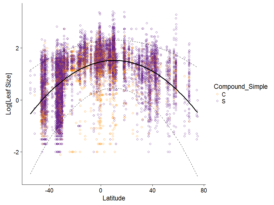
Let’s recreate the plot in Wright et al (more or less)

#  Leaf Size ~ Latitude

ggplot(data = global, aes(x = Latitude, y = log10(Leaf.size)))+
        
    geom_point(pch = 1, aes(color = Compound_Simple), alpha = 0.7) + 
    
    scale_color_manual(values = c("darkorange", "darkorchid4")) + 
    
    geom_smooth(method = 'lm', formula = y ~ poly(x, 2), color = "black", se = F) + 
    
    ylab("Log[Leaf Size]") + 
    
    geom_quantile(quantiles  = c(0.05, 0.95),formula = y ~ poly(x, 2), lty = 2, color = "black")

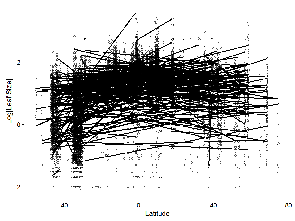
Now let’s plot Latitude against leaf size, but with separate lines for each family (we’ll use straight lines here, and take out the simple-compound coloring)

# Leaf Size ~ Latitude by family

ggplot(data = global, aes(x = Latitude, y = log10(Leaf.size)))+
        
    geom_point(pch = 1, alpha = 0.7) + 
    
    ylab("Log[Leaf Size]") + 
    
    geom_smooth(method = 'lm', formula = y~x, aes(group = Family), color = "black", se = F)

References

Wright IJ, Dong N, Maire V, Prentice IC, Westoby M, Díaz S, Gallagher R. 2017. Global climatic drivers of leaf size. Science, 357, 917-921. DOI: 10.1126/science.aal4760

Session Information

R version 3.4.2 (2017-09-28)
Platform: x86_64-w64-mingw32/x64 (64-bit)
Running under: Windows 7 x64 (build 7601) Service Pack 1

Matrix products: default

locale:
[1] LC_COLLATE=English_United States.1252 
[2] LC_CTYPE=English_United States.1252   
[3] LC_MONETARY=English_United States.1252
[4] LC_NUMERIC=C                          
[5] LC_TIME=English_United States.1252    

attached base packages:
[1] stats     graphics  grDevices utils     datasets  methods   base     

other attached packages:
 [1] quantreg_5.33 SparseM_1.77  bindrcpp_0.2  knitr_1.20    MuMIn_1.40.0 
 [6] lme4_1.1-17   Matrix_1.2-11 readxl_1.0.0  dplyr_0.7.4   cowplot_0.7.0
[11] ggplot2_2.2.1

loaded via a namespace (and not attached):
 [1] Rcpp_0.12.17       highr_0.6          nloptr_1.0.4      
 [4] pillar_1.1.0       compiler_3.4.2     cellranger_1.1.0  
 [7] plyr_1.8.4         bindr_0.1          prettydoc_0.2.1   
[10] tools_3.4.2        digest_0.6.15      evaluate_0.10     
[13] tibble_1.4.2       gtable_0.2.0       nlme_3.1-131      
[16] lattice_0.20-35    pkgconfig_2.0.1    rlang_0.2.0       
[19] yaml_2.1.19        stringr_1.3.0      MatrixModels_0.4-1
[22] stats4_3.4.2       rprojroot_1.2      grid_3.4.2        
[25] glue_1.2.0         R6_2.2.1           rmarkdown_1.9     
[28] minqa_1.2.4        magrittr_1.5       codetools_0.2-15  
[31] backports_1.1.2    scales_0.5.0       htmltools_0.3.6   
[34] splines_3.4.2      MASS_7.3-50        assertthat_0.2.0  
[37] colorspace_1.3-2   labeling_0.3       stringi_1.1.7     
[40] lazyeval_0.2.1     munsell_0.4.3     

RE: Global climatic drivers of leaf size

Anlaysis of trends in global leaf size data